System Reliability#
Pystra separates the system failure event from its probability calculation.
The pystra.system topology classes compose component limit states for
simulation. SystemFORM estimates series and parallel probabilities from
separate component FORM analyses in one shared standard-normal space.
Do not use ordinary FORM or SORM on the combined min/max function as a general system reliability method. One tangent plane can miss other failure regions, and ties can give misleading or zero finite-difference gradients.
The sign convention is the usual Pystra convention: positive values are safe and negative values indicate failure.
Series and Parallel Systems#
A series system fails when any child component or subsystem fails. Its equivalent limit-state value is therefore
A parallel system fails only when all child components or subsystems fail. Its equivalent limit-state value is therefore
Systems can be nested, so a user can describe a known structural topology without enumerating every failure path manually. This includes common branch system benchmarks such as the four-branch series example.
Original-system Monte Carlo#
import pystra as ra

system = ra.SeriesSystem(
    [
        ra.Component("flexure", lambda R, S: R - S),
        ra.Component("shear", lambda V, S: V - 2.0 * S),
        ra.ParallelSystem(
            [
                ra.Component("backup_a", lambda A: A),
                ra.Component("backup_b", lambda B: B),
            ]
        ),
    ],
    name="frame",
)

limit_state = system.as_limit_state()

model = ra.StochasticModel()
model.addVariable(ra.Normal("R", 10.0, 1.0))
model.addVariable(ra.Normal("V", 12.0, 1.0))
model.addVariable(ra.Normal("S", 4.0, 1.0))
model.addVariable(ra.Normal("A", 1.0, 0.5))
model.addVariable(ra.Normal("B", 1.0, 0.5))

import numpy as np

options = ra.AnalysisOptions()
options.setSamples(100_000)  # maximum budget; may stop at target CoV
options.setPrintOutput(False)
np.random.seed(2026)
mc = ra.CrudeMonteCarlo(
    stochastic_model=model, limit_state=limit_state,
    analysis_options=options,
)
mc.run()
print(mc.getFailure(), mc.cov_q_bar[mc.k - 1], mc.k)
Monte Carlo evaluates the original nonlinear failure event, including mixed and cut/tie-set topologies. The reported CoV describes sampling uncertainty. Zero observed failures do not establish a zero failure probability: increase the sample budget or use a validated rare-event method. The legacy Monte Carlo beta value is not meaningful when no failures are observed.
Component functions may use only the stochastic variables they need. Extra model variables are filtered at the component boundary, which keeps small component functions reusable inside larger systems.
Component-based system FORM#
from scipy.stats import norm

model = ra.StochasticModel()
model.addVariable(ra.Normal("X", 0.0, 1.0))
model.addVariable(ra.Normal("Y", 0.0, 1.0))
components = [
    ra.Component("a", lambda X: 3.0 - X),
    ra.Component("b", lambda Y: 3.0 - Y),
]
analysis = ra.SystemFORM(ra.SeriesSystem(components), model)
analysis.run()
print(analysis.getFailure())  # approximately 0.002697974
print(analysis.getBeta())     # equivalent system index
print(analysis.bounds)        # Ditlevsen bounds on the linearized event
print(analysis.correlation)   # correlations of normal scores
print(analysis.component_results["a"].getDesignPoint())

p = norm.sf(3.0)
assert abs(analysis.getFailure() - (2*p - p*p)) < 1e-10
Use ParallelSystem(components) for joint failure; the exact result in this
example is p*p. Homogeneous nesting is flattened and shared component
objects are analysed once. Component names must be unique. Mixed topology,
k-of-n and cut/tie-set inputs are currently rejected by SystemFORM; use
original-system simulation for these events.
For each component, FORM finds a tangent failure half-space in the same independent standard-normal coordinates:
This includes dependence caused by shared variables and the Nataf input
correlation model. correlation is the correlation of the linearized normal
scores, not of the physical variables or binary failure indicators. All
components retain the full model variable order. DDM functions must return
gradients in that full order, including zeros for unused variables.
component_results retains the individual Form objects, including
converged, e1 and e2 diagnostics. A failed component analysis raises
an error and leaves the system result invalid. Ordinary Form now warns
when it exhausts its iterations, and marks results_valid false.
Series probabilities are integrated as disjoint first-failure events, avoiding
subtraction of an almost-unit survival probability. Parallel probabilities
use the joint normal failure event. Singular component correlation matrices
are supported. maxpts, abseps and releps control integration effort
and requested tolerances; they do not certify numerical accuracy in rare
multivariate tails. Bivariate integration uses relative-tolerance quadrature.
Check sensitivity to tighter tolerances for demanding problems.
Series results include Ditlevsen bounds and intersections. Parallel results
include the marginal/Frechet bounds. These bounds apply to the linearized
events, with numerically evaluated probabilities. They are not guaranteed
bounds on the original nonlinear system. Component FORM may also find a local
design point; convergence alone does not establish global accuracy.
The method is exact up to integration error for affine limit states in standard-normal space. For nonlinear components, compare with original-system simulation. The four-branch notebook illustrates the difference between the first-order approximation and the nonlinear event probability.
Event Topologies#
Structural systems are often specified as event logic once the engineer has identified the relevant component limit states. Pystra provides three small helpers for that layer:
KofNSystemfails when at least
kchildren fail.KofNSystem(children, k=1)has the same failure event as a series system, andKofNSystem(children, k=n)has the same failure event as a parallel system.CutSetSystemfails when any supplied cut set has fully failed. This is useful when the user already knows the minimal cut sets of the structure.
TieSetSystemremains safe when any supplied tie set remains fully safe. This is useful for path-based descriptions of redundant systems.
For example, Song and Der Kiureghian’s rigid-plastic cantilever-bar benchmark has the system failure event
This can be represented directly from named components:
components = {
    "E1": ra.Component("E1", lambda T, X: T - 5.0 * X / 16.0),
    "E2": ra.Component("E2", lambda M, L, X: M - L * X),
    "E3": ra.Component("E3", lambda M, L, X: M - 3.0 * L * X / 8.0),
    "E4": ra.Component("E4", lambda M, L, X: M - L * X / 3.0),
    "E5": ra.Component("E5", lambda M, L, T, X: M + 2.0 * L * T - L * X),
}

system = ra.CutSetSystem(
    [["E1", "E2"], ["E3", "E4"], ["E3", "E5"]],
    components=components,
)
These topologies preserve the failure sign for direct Monte Carlo and Boolean enumeration. The current k-of-n performance function is a discrete count; its plateaus make it unsuitable as a general subset-simulation performance measure. Existing line sampling assumes one failure tail per line, and existing importance sampling uses one FORM design point. Neither should be assumed to cover arbitrary system failure regions.
Ditlevsen Bounds#
When component event probabilities and pairwise intersection probabilities are
available, pystra.ditlevsen_bounds() computes Ditlevsen’s
second-order bounds for a union of failure
events. The event ordering can be supplied explicitly, or exhaustively
optimized for small systems. Every pair must be supplied (explicit zero for
disjoint events); nonfinite values and violations of marginal/Frechet bounds
are rejected. These checks do not prove global consistency of all supplied
probabilities.
probabilities = [0.1, 0.2]
intersections = {(0, 1): 0.03}

lower, upper = ra.ditlevsen_bounds(probabilities, intersections)
For two events the bounds collapse to the exact inclusion-exclusion result.
For larger systems they provide a cheap check on simulation estimates and a
useful validation target for future system FORM approximations. The initial
test suite includes Mainçon’s identical 100-element series benchmark, where the Ditlevsen
upper bound is approximately 6.216e-2.
Scope and Transformations#
The system module composes limit-state functions in the original physical
variables. The isoprobabilistic transformation to standard space remains the
responsibility of the selected Pystra analysis method and its
AnalysisOptions. This keeps system topology separate from the probability
transformation, following the same conceptual split used in structural
reliability methods generally.
SystemFORM uses Pystra’s existing Nataf transformation, with the same
factorisation choice for every component. Automatic failure-path enumeration,
load redistribution and importance sampling around multiple design points
remain future extensions.
Validation Benchmarks#
The current validation suite checks exact Boolean behaviour for series,
parallel, k-of-n, cut-set, and tie-set systems; integration with Pystra’s
LimitState evaluation; independent and correlated linear system
probabilities; identical and opposing component directions; positive rescaling;
shared components; failed FORM diagnostics; and Ditlevsen input validation.
The legacy combined-limit-state FORM smoke test checks execution only, not
system probability accuracy.
The next benchmarks to add before extending the approximation methods are:
Song and Der Kiureghian’s rigid-plastic cantilever-bar cut-set example and linear-programming bounds;
Mainçon’s correlated series-system cases and related equivalent planes comparisons.