Theoretical Background#

Structural Reliability#

Structural reliability analysis (SRA) is an important part to handle structural engineering applications. This section provides a brief introduction to this topic and is also the theoretical background for the Python library, Python Structural Reliability Analysis (Pystra).

Limit States#

The word structural reliability refers to the meaning “how much reliable is a structure in terms of fulfilling its purpose” [Malioka2009]. The performance of structures and engineering systems was based on deterministic parameters even for a long time, even if it was known that all stages of the system involve uncertainties. SRA provides a method to take those uncertainties into account in a consistent manner. In this content the term probability of failure is more common than reliability. [Malioka2009]

In general, the term “failure” is a vague definition because it means different things in different cases. For this purpose the concept of limit state is used to define failure in the context of SRA. [Nowak2000]

Note

A limit state represents a boundary between desired and undesired performance of a structure.

This boundary is usually interpreted and formulated within a mathematical model for the functionality and performance of a structural system, and expressed by a limit state function. [Ditlevsen2007]

Note

[Limit State Function]

Let \({\bf X}\) describe a set of random variables \({X}_1 \dots {X}_n\) which influence the performance of a structure. Then the functionality of the structure is called limit state function, denoted by \(g\) and given by

(1)#\[ g({\bf X})=g(X_1,\dots,X_n)\]

The boundary between desired and undesired performance would be given when \(g({\bf X}) = 0\). If \(g({\bf X}) > 0\), it implies a desired performance and the structure is safe. An undesired performance is given by \(g({\bf X}) \leq 0\) and it implies an unsafe structure or failure of the system. [Baker2010]

The probability of failure \(p_f\) is equal to the probability that an undesired performance will occur. It can be mathematical expressed as

(2)#\[ p_f = P(g({\bf X})\leq 0) = \iiint\limits_{g({\bf X})\leq 0} f_{{\bf X}}({\bf x}) d {\bf x}\]

assuming that all random variables \({\bf X}\) are continuous. However, there are three major issues related to the Equation (2), proposed by [Baker2010]:

There is not always enough information to define the complete joint probability density function \(f_X({\bf x})\).

The limit state function \(g({\bf X})\) may be difficult to evaluate.

Even if \(f_X({\bf x})\) and \(g({\bf X})\) are known, numerical computing of high dimensional integrals is difficult.

For this reason various methods have been developed to overcome these chal- lenges. The most common ones are the Monte Carlo simulation method and the First Order Reliability Method (FORM).

The Classical Approach#

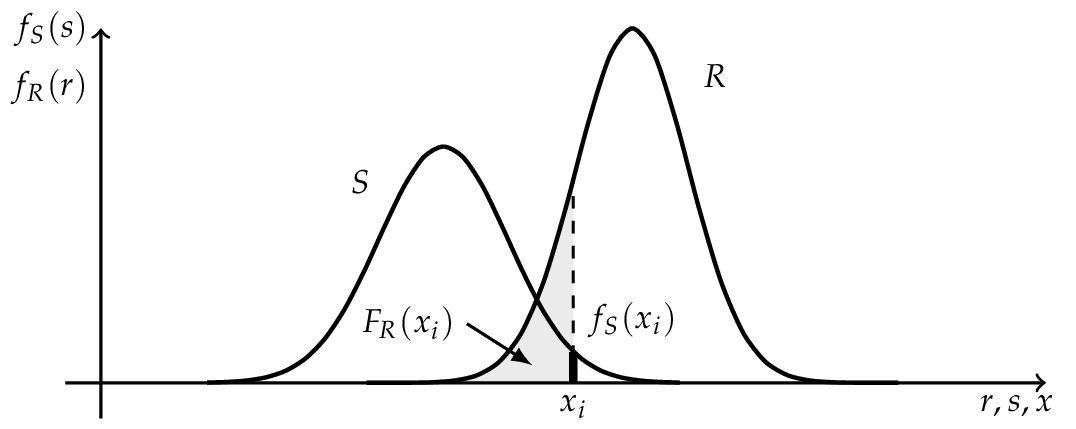
Before discussing more general methods, the principles are shown on a “historical” and simplified limit state function.

(3)#\[ g(R,S) = R - S\]

Where \(R\) is a random variable for the resistance with the outcome \(r\) and \(S\) represents a random variable for the internal strength or stress with the outcome of \(s\). [Lemaire2010] The probability of failure is according to Equation (2):

(4)#\[ p_f = P(R-S \leq 0) = \iint\limits_{r\leq s} f_{R,S}(r,s) d r d s\]

If \(R\) and \(S\) are independent the Equation (4) can be rewritten as a convolution integral, where the probability of failure \(p_f\) can be (numerical) computed. [Schneider2007]

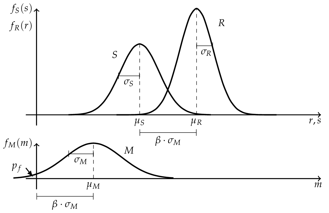
(5)#\[ p_f = P(R-S \leq 0) = \int_{-\infty}^{\infty} F_R(x) f_{S}(x) d x\]

If \(R\) and \(S\) are independent and \(R \sim N (\mu_R , \sigma_R )\) as well as \(S \sim N (\mu_S , \sigma_S )\) are normally distributed, the convolution integral (5) can be evaluated analytically.

(6)#\[ M = R - S\]

where \(M\) is the safety margin and also normal distributed \(M \sim N (\mu_M , \sigma_M )\) with the parameters

(7)#\[ \mu_M = \mu_R-\mu_S\]

(8)#\[ \sigma_M = \sqrt{\sigma_R^2+\sigma_S^2}\]

The probability of failure \(p_f\) can be determined by the use of the standard normal distribution function.

(9)#\[ p_f = \Phi\left(\frac{0-\mu_m}{\sigma_M}\right)=\Phi(-\beta)\]

Where \(\beta\) is the so called Cornell reliability index, named after Cornell (1969), and is equal to the number of the standard derivation \(\sigma_M\) by which the mean values \(\mu_M\) of the safety margin \(M\) are zero. [Faber2009]

Hasofer and Lind Reliability Index#

The reliability index can be interpreted as a measure of the distance to the failure surface, as shown in the Figure above. In the one dimensional case the standard deviation of the safety margin was used as scale. To obtain a similar scale in the case of more basic variables, Hasofer and Lind (1974) proposed a non-homogeneous linear mapping of a set of random variables \({\bf X}\) from a physical space into a set of normalized and uncorrelated random variables \({\bf Z}\) in a normalized space. [Madsen2006]

Note

[Hasofer and Lind Reliability Index]

The Hasofer and Lind reliability index, denoted by \(\beta_{HL}\), is the shortest distance \({\bf z}^*\) from the origin to the failure surface \(g({\bf Z})\) in a normalized space.

(10)#\[ \beta_{HL}:=\beta={\vec\alpha}^T{\bf z}^*\]

The shortest distance to the failure surface \({\bf z}^*\) is also known as design point and \({\vec \alpha}\) denotes the normal vector to the failure surface \(g({\bf Z})\) and is given by

(11)#\[ {\vec\alpha} = - \frac{\nabla g({\bf z}^*)}{|\nabla g({\bf z}^*)|}\]

where \(g({\bf z})\) is the gradient vector, which is assumed to exist: [Madsen2006]

(12)#\[ \nabla g({\bf z}) = \left (\frac{\partial g}{\partial z_1}({\bf z}),\ldots, \frac{\partial g}{\partial z_n}({\bf z})\right)\]

Finding the reliability index \(\beta\) is therefore an optimization problem

(13)#\[ \min_x \, |{\bf z}|\,: \, g({\bf z})=0\]

The calculation of \(\beta\) can be undertaken in a number of different ways. In the general case where the failure surface is non-linear, an iterative method must be used. [Thoft-Christensen]

Probability Transformation#

Due to the reliability index \(\beta_{HL}\) , being only defined in a normalized space, the basic random variables \(\bf X\) have to be transformed into standard normal random variables \(\bf Z\). Additionally, the basic random variables \(\bf Z\) can be correlated and those relationships should also be transformed.

Transformation of Dependent Random Variables using Nataf Approach#

One method to handle this is using the Nataf joint distribution model, if the marginal cdfs are known. [Baker2010] The correlated random variables \({\bf X} = ( X_1 , \dots , X_n )\) with the correlation matrix \(\bf R\) can be transformed by

(14)#\[ y_i=\Phi^{-1}\left(F_{X_{i}}(x_i)\right) \qquad i = 1,\dots,n\]

into normally distributed random variables \(\bf Y\) with zero means and unit variance, but still correlated with \({\bf R}_0\) . Nataf’s distribution for \(\bf X\) is obtained by assuming that \(\bf Y\) is jointly normal. [Liu1986]

The correlation coefficients for \(\bf X\) and \(\bf Y\) are related by

(15)#\[ \rho_{X_i,X_j} = \int\limits_{-\infty}^{\infty}\int\limits_{-\infty}^{\infty} \left(\frac{x_i-\mu_{X_i}}{\sigma_{X_i}}\right) \left(\frac{x_j-\mu_{X_j}}{\sigma_{X_j}}\right) \frac{1}{2\pi \sqrt{1-\rho_{Y_i,Y_j}^2}} \exp\left(-\frac{y_i^2-2\rho_{Y_i,Y_j}y_iy_j+y_j^2}{2(1-\rho_{Y_i,Y_j}^2)}\right) d z_i d z_j\]

Once this is done, the transformation from the correlated normal random variables \(\bf Y\) to uncorrelated normal random variables \(\bf Z\) is addressed. Hence, the transformation is

(16)#\[ {\bf z}={\bf L}_0^{-1}{\bf y} \quad \Leftrightarrow \quad {\bf y} = {\bf L}_0{\bf z}\]

where \(\bf L\) is the Cholesky decomposition of the correlation matrix \(\bf R\) of \(\bf Y\). The Jacobian matrix, denoted by \(\bf J\), for the transformation is given by

(17)#\[ {\bf J}_{ZX} = \frac{\partial {\bf z}}{\partial {\bf x}} = {\bf L}_0^{-1}\text{diag} \left(\frac{f_{X_i}(x_i)}{\Phi (z_i)}\right)\]

This approach is useful when the marginal distribution for the random variables \(\bf X\) is known and the knowledge about the variables dependence is limited to correlation coefficients. [Baker2010]

Transformation of Dependent Random Variables using Rosenblatt Approach#

An alternative to the Nataf approach is to consider the joint pdf of \(\bf X\) as a product of conditional pdfs.

(18)#\[ f_{{\bf X}}({\bf x}) = f_{X_1}(x_1) f_{X_2|X_1}(x_2|x_1) \dots f_{X_n|X_1,\dots,X_{n-1}}(x_n|x_1,\dots,x_{n-1})\]

As a result of the sequential conditioning in the pdf, the conditional cdfs are given for \(i \in [1,n]\)

(19)#\[ F_{X_i|X_1,\dots,X_{i-1}}(x_i|x_1,\dots,x_{i-1}) = \int_{-\infty}^{x_i} f_{X_i|X_1,\dots,X_{i-1}}(x_i|x_1,\dots,x_{i-1}) d x_i\]

These conditional distributions for the random variables \(\bf X\) can be transformed into standard normal marginal distributions for the variables \(\bf Z\), using the so called Rosenblatt transformation [Rosenblatt1952], suggested by Hohenbichler and Rackwitz (1981).

(20)#\[\begin{split} \begin{split} z_1 &= \Phi^{-1}\left( F_{X_1}(x_1) \right)\\ z_2 &= \Phi^{-1}\left( F_{X_2|X_1}(x_2|x_1) \right)\\ &\vdots\\ z_n &= \Phi^{-1}\left( F_{X_n|X_1,\dots,X_{n-1}}(x_n|x_1,\dots,x_{n-1}) \right) \end{split}\end{split}\]

The Jacobian of this transformation is a lower triangular matrix having the elements [Baker2010]

(21)#\[\begin{split} \left[{\bf J}_{ZX}\right]_{i,j} = \frac{\partial z_i}{\partial x_j} = \begin{cases}\displaystyle \frac{1}{\Phi(u_i)}\frac{\partial}{\partial x_j} F_{X_i|X_1,\dots,X_{i-1}}(x_i|x_1,\dots,x_{i-1}) & i \geq j\\ 0 & i < j \end{cases}\end{split}\]

In some cases the Rosenblatt transformation cannot be applied, because the required conditional pdfs cannot be provided. In this case other transformations may be useful, for example Nataf transformation. [Faber2009]

First-Order Reliability Method (FORM)#

Let \(\bf Z\) be a set of uncorrelated and standardized normally distributed random variables \(( Z_1 ,\dots, Z_n )\) in the normalized z-space, corresponding to any set of random variables \({\bf X} = ( X_1 , \dots , X_n )\) in the physical x-space, then the limit state surface in x-space is also mapped on the corresponding limit state surface in z-space.

According to Definition (10), the reliability index \(\beta\) is the minimum distance from the z-origin to the failure surface. This distance \(\beta\) can directly be mapped to a probability of failure

(22)#\[ p_f \approx p_{f1} = \Phi(-\beta)\]

this corresponds to a linearization of the failure surface. The linearization point is the design point \({\bf z}^*\). This procedure is called First Order Reliability Method (FORM) and \(\beta\) is the First Order Reliability Index. [Madsen2006]

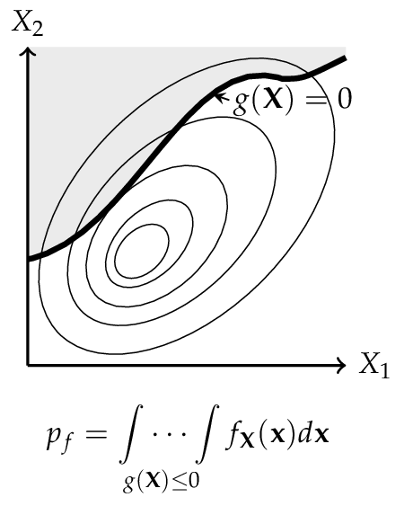
Representation of a physical space with a set \({\bf X}\) of any two random variables. The shaded area denotes the failure domain and \(g({\bf X}) = 0\) the failure surface.

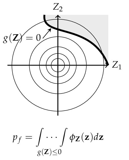
After transformation in the normalized space, the random variables \({\bf X}\) are now uncorrelated and standardized normally distributed, also the failure surface is transformed into \(g({\bf Z}) = 0\).

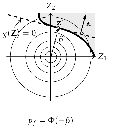
FORM corresponds to a linearization of the failure surface \(g({\bf Z}) = 0\). Performing this method, the design point \({\bf z}^*\) and the reliability index \(\beta\) can be computed.

Second-Order Reliability Method (FORM)#

Better results can be obtained by higher order approximations of the failure surface. The Second Order Reliability Method (SORM) uses; for example, a quadratic approximation of the failure surface. [Baker2010]

Simulation Methods#

The preceding sections describe some methods for determining the reliability index \(\beta\) for some common forms of the limit state function. However, it is sometimes extremely difficult or impossible to find \(\beta\). [Nowak2000]

In this case, Equation (2) may also be estimated by numerical simulation methods. A large variety of simulation techniques can be found in the literature, indeed, the most commonly used method is the Monte Carlo method. [Faber2009]

The principle of simulation methods is to carry out random sampling in the physical (or standardized) space. For each of the samples the limit state function is evaluated to figure out, whether the configuration is desired or undesired. The probability of failure \(p_f\) is estimated by the number of undesired configurations, respected to the total numbers of samples. [Lemaire2010]

For this analysis Equation (2) can be rewritten as

(23)#\[ p_f = P(g({\bf X})\leq 0) = \iiint\limits_{g({\bf X})\leq 0} I(g({\bf X})\leq 0) f_{{\bf X}}({\bf x}) d {\bf x}\]

where \(I\) is an indicator function that is equals to 1 if \(g({\bf X}) \leq 0\) and otherwise 0. Equation (23) can be interpreted as expected value of the indicator function. Therefore, the probability of failure can be estimated such as [Malioka2009]

(24)#\[ \tilde{p}_f = \text{Ex}\left[I(g({\bf X})\leq 0)\right] = \frac{1}{n}\sum_{i=1}^{n} I(g({\bf X})\leq 0)\]

Crude Monte Carlo Simulation#

The Crude Monte Carlo simulation (CMC) is the most simple form and corresponds to a direct application of Equation (24). A large number \(n\) of samples are simulated for the set of random variables \(\bf X\). All samples that lead to a failure are counted \(n_f\) and after all simulations the probability of failure \(p_f\) may be estimated by [Faber2009]

(25)#\[ \tilde{p}_f = \frac{n_f}{n}\]

Theoretically, an infinite number of simulations will provide an exact probability of failure. However, time and the power of computers are limited; therefore, a suitable amount of simulations \(n\) are required to achieve an acceptable level of accuracy. One possibility to reach such a level is to limit the coefficient of variation CoV for the probability of failure. [Lemaire2010]

(26)#\[ \text{CoV} = \sqrt{\frac{1-p_f}{n p_f}} \approx \frac{1}{\sqrt{n p_f}} \qquad \text{for} \quad p_f \to 0\]

Importance Sampling#

To decrease the number of simulations and the coefficient of variation, other methods can be performed. One commonly applied method is the Importance Sampling simulation method (IS). Here the prior information about the failure surface is added to Equation (23)

(27)#\[ p_f = P(g({\bf X})\leq 0) = \iiint\limits_{g({\bf X})\leq 0} I(g({\bf X})\leq 0) \frac{f_{{\bf X}}({\bf x})}{h_{{\bf X}}({\bf x})} h_{{\bf X}}({\bf x}) d {\bf x}\]

where \(h_{X} ({\bf X})\) is the importance sampling probability density function of \(\bf X\). Consequently Equation (24) is extended to [Faber2009]

(28)#\[ \tilde{p}_f = \text{Ex}\left[I(g({\bf X})\leq 0) \frac{f_{{\bf X}}({\bf x})}{h_{{\bf X}}({\bf x})}\right] = \frac{1}{n}\sum_{i=1}^{n} I(g({\bf X})\leq 0)\frac{f_{{\bf X}}({\bf x})}{h_{{\bf X}}({\bf x})}\]

The key to this approach is to choose \(h_{X} ({\bf X})\) so that samples are obtained more frequently from the failure domain. For this reason, often a FORM (or SORM) analysis is performed to find a prior design point. [Baker2010]

Representation of a physical space with a set \({\bf X}\) of any two random variables. The shaded area denotes the failure domain and g({bf X}) = 0 the failure surface.

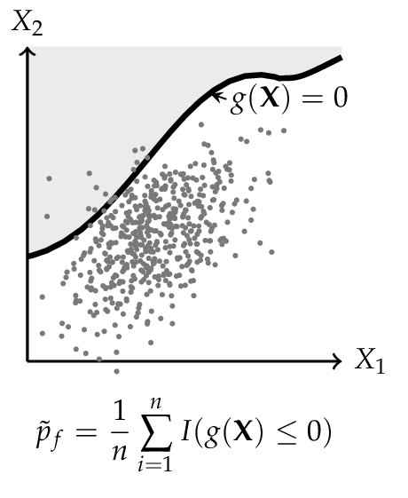
For the CMC method every dot corresponds to one configuration of the random variables \({\bf X}\). Dots in shaded areas lead to a failure.

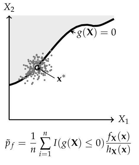
The IS simulation method uses a distribution centered on the design point \({\bf x}^*\), is obtained from a FORM (or SORM) analysis. More dots in the failure domain can be observed.