Load Combinations

Pystra includes the class LoadCombination for named structural reliability cases. A load combination case is an explicit mapping from limit-state variables to ordinary Pystra distributions or constants. This keeps the mechanics visible while still providing convenience methods for building stochastic models and running FORM.

Example

This demonstration problem is adapted from Example 4, pp. 190-191, in Sørensen (2004). The parameter values are slightly modified for demonstration.

Import Libraries

import pystra as ra
import numpy as np
import pandas as pd
from matplotlib import pyplot as plt

Define the limit state function

The LSF supplied to LoadCombination can be any valid Pystra LSF. Here the deterministic coefficient cg is kept as an explicit input.

def lsf(R, G, Q1, Q2, cg):
    return R - (cg*G + 0.8*Q1 + 0.2*Q2)

Define the load and resistance distributions

Start by defining the distributions that represent the structural reliability model. In this first example we use explicit annual-maximum and point-in-time distributions so that each load case can state exactly which distribution is used.

Define the annual max distributions

Q1max = ra.Gumbel("Q1", 1, 0.2)  # Imposed Load
Q2max = ra.Gumbel("Q2", 1, 0.4)  # Wind Load

Next specify inferred point-in-time distributions. These are ordinary Pystra distributions and can be inspected or used directly.

Q1pit = ra.Gumbel("Q1", 0.89, 0.2)  # Imposed Load
Q2pit = ra.Gumbel("Q2", 0.77, 0.4)  # Wind Load

Define the deterministic coefficient used by the LSF.

cg = ra.Constant("cg", 0.4)

Finally, define any other random variables in the problem

Rdist = ra.Lognormal("R", 2.0, 0.15)  # Resistance
Gdist = ra.Normal("G", 1, 0.1)  # Permanent Load (Other load variable)

Specify explicit load-combination cases

A LoadCombination is now most clearly written as named explicit cases. Each case contains the actual variables used in that reliability analysis. This avoids hiding structural reliability assumptions inside a max/pit switching dictionary.

The Q1_leading and Q2_leading cases are Turkstra-style leading-action cases. The Q1Q2_max case is also shown as a deliberately conservative comparison where both variable actions are taken as annual maxima.

cases = {
    "Q1Q2_max": {"R": Rdist, "G": Gdist, "Q1": Q1max, "Q2": Q2max},
    "Q1_leading": {"R": Rdist, "G": Gdist, "Q1": Q1max, "Q2": Q2pit},
    "Q2_leading": {"R": Rdist, "G": Gdist, "Q1": Q1pit, "Q2": Q2max},
}

Specify user-defined correlation (optional)

A correlation matrix can be supplied for the random variables in the reliability problem.

variable_names = ["Q1", "Q2", "R", "G"]
correlation_values = np.eye(len(variable_names))
correlation = pd.DataFrame(
    data=correlation_values,
    columns=variable_names,
    index=variable_names,
)
rho_q1_q2 = 0.8
correlation.loc["Q1", "Q2"] = rho_q1_q2
correlation.loc["Q2", "Q1"] = rho_q1_q2
print(correlation)

     Q1   Q2    R    G
Q1  1.0  0.8  0.0  0.0
Q2  0.8  1.0  0.0  0.0
R   0.0  0.0  1.0  0.0
G   0.0  0.0  0.0  1.0

Specify user-defined analysis options (optional)

Analysis options can be supplied in the usual Pystra way. In this tutorial we set error thresholds and change the default transform method to use singular value decomposition.

options = ra.AnalysisOptions()
options.setE1(1e-3)
options.setE2(1e-3)
options.setTransform("svd")

Instantiate LoadCombination

The explicit cases mapping is the canonical interface. The remaining arguments are the limit-state function and optional analysis inputs.

lc = ra.LoadCombination(
    lsf=lsf,
    cases=cases,
    constants=[cg],
    corr=correlation,
    opt=options,
)

Inspect the generated stochastic models

Because the cases are explicit, they can be inspected before any analysis is run.

for name in lc.get_label("comb_cases"):
    print(name, list(lc.case(name).keys()))

Q1Q2_max ['R', 'G', 'Q1', 'Q2']
Q1_leading ['R', 'G', 'Q1', 'Q2']
Q2_leading ['R', 'G', 'Q1', 'Q2']

Analyse load cases

Run FORM for each named case.

form = {}
for name in lc.get_label("comb_cases"):
    form[name] = lc.run_reliability_case(lcn=name)

Detailed output for one load case

form["Q1_leading"].showDetailedOutput()

==========================================================
FORM
==========================================================
Pf                       1.9624337657e-02
BetaHL                   2.0615701821
Model Evaluations        49
----------------------------------------------------------
Variable            U_star             X_star        alpha
R                -1.926554           1.896315    -0.934503
G                -0.673345           1.018964    -0.326631
Q1                0.189636           1.461699    +0.091993
Q2               -0.221604           1.596853    -0.107490
cg                     ---           0.400000          ---
==========================================================

Display reliability per load combination

for name, result in form.items():
    print(f"{name}: β = {result.getBeta():.2f}")

Q1Q2_max: β = 1.95
Q1_leading: β = 2.06
Q2_leading: β = 2.16

Ferry-Borges-Castanheta process model

For variable actions represented by a Ferry-Borges-Castanheta rectangular-wave process, use FBCProcess to expose the process assumptions. The FBC process defines the load magnitude distributions. Turkstra’s rule defines the combination cases: each variable action is considered as leading in turn, while the others are taken as companion actions. In this context a companion action may be a point-in-time value or an intermediate maximum over the leading action’s interval.

In Sørensen’s imposed-load/wind example the reference period is T = 1 year. The imposed load has tau_1 = 0.5 years, so r_1 = T / tau_1 = 2. The wind load has tau_2 = 1 / 360 years, so r_2 = T / tau_2 = 360. These recurrence counts describe the underlying FBC process; they are not load-combination factors.

The easy mistake is to look at the companion wind distribution and conclude that wind has somehow become an r = 2 process. It has not. If Q1 is leading, Turkstra’s rule takes Q2 as the maximum over the Q1 interval tau_1. That interval contains r_2 / r_1 = 180 wind intervals. Written in terms of the annual-maximum wind distribution, this gives F_Q2C = F_Q2,max ** (1 / r_1) = F_Q2,max ** 0.5. The wind process still has r_2 = 360; the companion wind value is a half-year maximum.

reference_period = 1.0
tau_1 = 0.5
tau_2 = 1 / 360

Q1_process = ra.FBCProcess.from_maximum(
    "Q1", maximum=Q1max, maximum_duration=reference_period, basic_interval=tau_1
)
Q2_process = ra.FBCProcess.from_maximum(
    "Q2", maximum=Q2max, maximum_duration=reference_period, basic_interval=tau_2
)

turkstra_lc = ra.LoadCombination.turkstra(
    lsf=lsf,
    resistance={"R": Rdist},
    permanent={"G": Gdist},
    variable={"Q1": Q1_process, "Q2": Q2_process},
    constants=[cg],
    reference_period=reference_period,
    corr=correlation,
    opt=options,
)

for name in turkstra_lc.get_label("comb_cases"):
    case = turkstra_lc.case(name)
    print(f"{name}:")
    for load in ("Q1", "Q2"):
        print(f"  {load}: {case[load].dist_type}, FBC intervals = {case[load].N:.2f}")

Q1_leading:
  Q1: Maximum, FBC intervals = 2.00
  Q2: Maximum, FBC intervals = 180.00
Q2_leading:
  Q1: Maximum, FBC intervals = 1.00
  Q2: Maximum, FBC intervals = 360.00

The generated Turkstra cases can be analysed in exactly the same way as the manually specified cases.

turkstra_form = {}
for name in turkstra_lc.get_label("comb_cases"):
    turkstra_form[name] = turkstra_lc.run_reliability_case(lcn=name)

for name, result in turkstra_form.items():
    print(f"{name}: β = {result.getBeta():.2f}")

Q1_leading: β = 2.04
Q2_leading: β = 2.11

/home/runner/work/pystra/pystra/src/pystra/integration.py:49: RuntimeWarning: invalid value encountered in sqrt
  * (2 * np.pi * np.sqrt(1 - rho0**2)) ** (-1)
/home/runner/work/pystra/pystra/src/pystra/integration.py:50: RuntimeWarning: overflow encountered in exp
  * np.exp(

Distributions for Load Combinations

Pystra includes a range of tools to represent variable loads and load processes:

• Zero-Inflated distributions allow for a probability of non-occurrence of a load.

• Maximum distributions give the distribution of maxima of a supplied parent or point-in-time distribution.

• MaxParent distributions infer a parent distribution from a supplied maximum.

• FBCProcess wraps Maximum and MaxParent for Ferry-Borges-Castanheta rectangular-wave process modelling.

• LoadCombination.turkstra uses FBC process distributions to generate leading-action combination cases according to Turkstra’s rule.

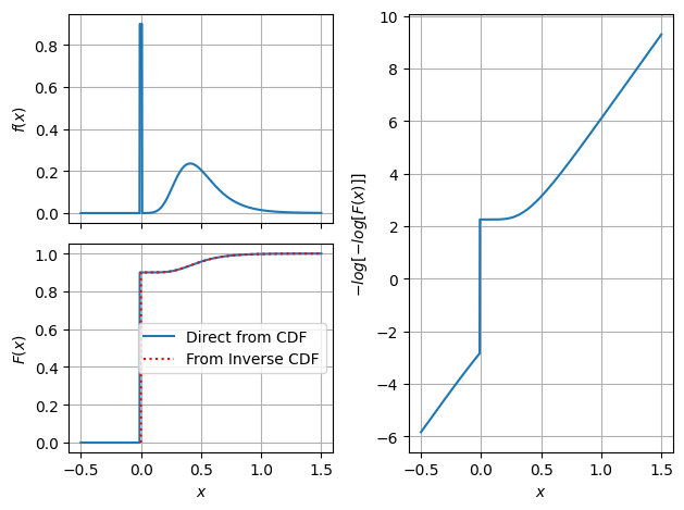
Zero-Inflated Distribution

zin = ra.ZeroInflated('Q',ra.Gumbel("G", 0.5, 0.2),p=0.9)
zin.zero_tol = 1e-2
x = np.linspace(-0.5,1.5,1000)
pdf = zin.pdf(x)
cdf = zin.cdf(x)
u = np.linspace(0,1,10001)
ppf = zin.ppf(u)
fig,axs = plt.subplot_mosaic([['a','c'],['b','c']],sharex=True)
ax = axs['a']
ax.plot(x,pdf)
ax.set_ylabel('$f(x)$')
ax.grid()
ax = axs['b']
ax.plot(x,cdf,label='Direct from CDF')
ax.plot(ppf,u,'r:',label='From Inverse CDF')
ax.set_ylabel('$F(x)$')
ax.set_xlabel('$x$')
ax.legend(loc='center right')
ax.grid()
ax = axs['c']
ax.plot(x,-np.log(-np.log(cdf)))
ax.set_ylabel('$-log[-log[F(x)]]$')
ax.set_xlabel('$x$')
ax.grid()
plt.tight_layout();
#fig.set_layout('tight');

Example

def lsf(R,G,Q):
    return R - (G + Q)

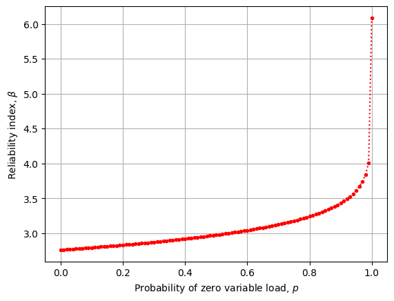
def reliability(p=0.0):
    ls = ra.LimitState(lsf)
    sm = ra.StochasticModel()
    sm.addVariable(ra.Lognormal("R", 6.0,0.15))
    sm.addVariable(ra.Normal("G", 4.5, 0.2))

    g = ra.Gumbel("Q", 0.5, 0.2)
    if p == 1.0:
        sm.addVariable(ra.Constant("Q",0.0))
    elif p == 0.0:
        sm.addVariable(g)
    else:
        zig = ra.ZeroInflated("Q",g,p=p)
        sm.addVariable(zig)

    form = ra.Form(sm,ls)
    form.run()

    return form

betas = []
ps = np.linspace(0,1.0,101)
for p in ps:
    form = reliability(p=p)
    betas.append(form.beta)

fig,ax = plt.subplots()
ax.plot(ps,betas,'r.:')
ax.set_xlabel('Probability of zero variable load, $p$')
ax.set_ylabel('Reliability index, $β$')
ax.grid();