Download notebook · Download runnable bundle

Dependencies: PySTRA core.

Code calibration using normalized reliability

Assess candidate code factors over representative load ratios using the normalized reliability approach. The workflow is: specify probability models and characteristic values, generate code-conforming designs, evaluate reliability, and compare the candidates against a target.

Before you start: the introductory reliability and load-combination tutorials. This example uses the core PySTRA installation.

Problem and assumptions

\(R\), \(G\), \(P\) and \(Q\) are normalized resistance, self-weight, other permanent load and variable load. Their means are one in this example; resistance and load model-error factors have separately specified means and variability.

The load ratios are \(a_g=G/(G+P)\) and \(a_q=Q/(G+P+Q)\), interpreted through the representative mean load contributions. Thus \(a_g=1\) means all permanent load is self-weight, while \(a_q=1\) means the demand is entirely variable load.

For each candidate factor set, solve the code equation for the resistance scale \(z\):

\[\phi z r_k=(1-a_q)\left[a_g\gamma_g g_k+(1-a_g)\gamma_p p_k\right]+a_q\gamma_q q_k.\]

Then assess the resulting design with

\[g=\omega_R z R-\omega_S\left[(1-a_q)\left(a_gG+(1-a_g)P\right)+a_qQ\right].\]

Here \(r_k,g_k,p_k,q_k\) are the normalized characteristic values. The model errors \(\omega_R\) and \(\omega_S\) multiply resistance and demand respectively. This is a dimensionless calibration study; the factor values and target below are illustrative inputs, not a prescribed design-code recommendation.

Specify the model and candidate factors

NormalizedReliabilityModel holds the probability model and characteristic values. CodeFactors describes one candidate code rule. Keeping those inputs separate makes comparisons between factor sets explicit.

import pystra as ra
import numpy as np
from dataclasses import replace

model = ra.calibration.NormalizedReliabilityModel(
    resistance_error=ra.Normal("wR", 1.06, 1.06 * 0.05),
    load_error=ra.Lognormal("wS", 1.0, 0.10),
    resistance=ra.Lognormal("R", 1.0, 0.08),
    dead_load=ra.Normal("G", 1.0, 0.08),
    permanent_load=ra.Normal("P", 1.0, 0.10),
    live_load=ra.Normal("Q", 1.0, 0.02),
    nominal_values=ra.calibration.NominalValues(
        resistance=1 / 1.08,
        dead_load=1 / 1.03,
        permanent_load=1.0,
        live_load=1 / 0.75,
    ),
)
current_factors = ra.calibration.CodeFactors(phi=0.80, gamma_g=1.2, gamma_p=1.7, gamma_q=1.6)
proposed_factors = replace(current_factors, gamma_p=1.5, gamma_q=1.4)

Evaluate code-conforming designs

CodeCalibration evaluates the load-ratio grid using the normalized reliability model. Each run returns the resistance scales, FORM results and margins against the target. Dependence can be supplied through NormalizedReliabilityModel.copula; this example uses independent inputs.

study = ra.calibration.CodeCalibration(
    live_load_ratios=np.arange(0.1, 1.1, 0.1),
    dead_load_ratios=np.arange(0.1, 1.1, 0.1),
)
current_result = study.run(model, current_factors, target_beta=4.7)
proposed_result = study.run(model, proposed_factors, target_beta=4.7)
assert current_result.converged and proposed_result.converged
current_result.to_frame().head()

	live_load_ratio	dead_load_ratio	design_value	failure_probability	beta	converged	status	message	method	target_margin
0	0.1	0.1	2.288503	7.290360e-09	5.666425	True	converged	Converged	FORM	0.966425
1	0.2	0.1	2.354225	1.183257e-09	5.970415	True	converged	Converged	FORM	1.270415
2	0.3	0.1	2.419947	1.789648e-10	6.271351	True	converged	Converged	FORM	1.571351
3	0.4	0.1	2.485669	2.575168e-11	6.566524	True	converged	Converged	FORM	1.866524
4	0.5	0.1	2.551391	3.631771e-12	6.852372	True	converged	Converged	FORM	2.152372

Compare reliability across the load ratios

The envelope spans the self-weight shares at each variable-load ratio. The dotted curve corresponds to the smallest self-weight share. plot_calibration consumes the completed results and identifies failed studies rather than hiding them.

results = {"Current": current_result, "Proposed": proposed_result}
fig, ax = ra.calibration.plot_calibration(
    results, target_beta=4.7, colors={"Current": "r", "Proposed": "g"}
)

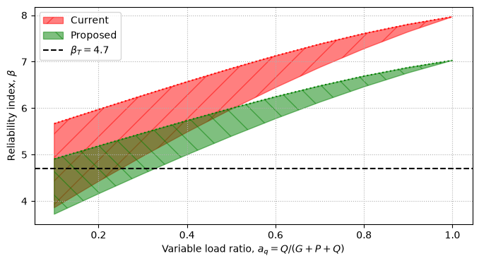
Figure. Current and proposed factor sets produce different reliability envelopes over live-load ratio. Compare each envelope with the target and inspect the full dead-load-ratio range.

Optional annotation ranges belong to the plotting call:

ranges = [
    {"xl": 0.2, "xu": 0.3, "ytext": 4.1, "text": "Footbridges", "alpha": 0.15},
    {"xl": 0.5, "xu": 0.65, "ytext": 4.1, "text": "Road Bridges", "alpha": 0.3},
    {"xl": 0.55, "xu": 0.75, "ytext": 4.8, "text": "Rail Bridges", "alpha": 0.4},
]
fig, ax = ra.calibration.plot_calibration(
    results, target_beta=4.7, ranges=ranges, colors={"Current": "r", "Proposed": "g"}
)

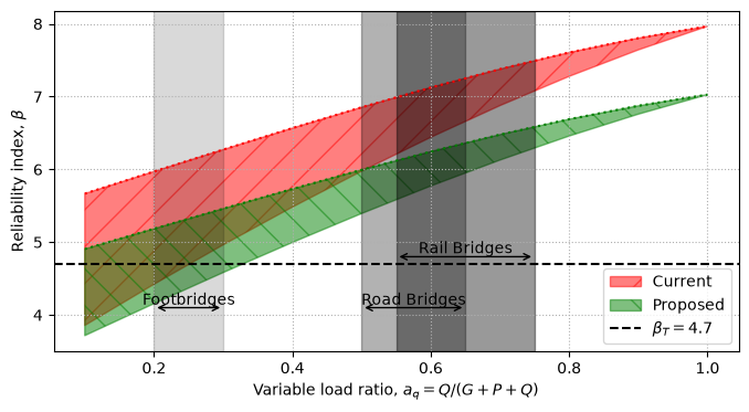
Figure. The same reliability comparison includes illustrative application ranges for footbridges, road bridges and rail bridges; these ranges are assumptions for the example.

Interpretation

Reducing load factors changes the resistance required by the code equation and therefore the achieved reliability. Inspect the per-case target margins before choosing a factor set. This example evaluates specified candidates; it does not automatically optimize the factors.

Calibrating partial and combination factors demonstrates factor derivation and verification within the same code-calibration workflow. See code-calibration theory for the normalized formulation and its relationship to those operations.

Study results retain every grid point. Inspect current_result.converged and the status/message columns of current_result.to_frame() before comparing factor sets. An alternative reliability method or external adapter can be supplied with evaluator=; see the calibration guide.

Continue: User guide · API reference · Theory