Download notebook · Download runnable bundle

Dependencies: PySTRA core.

Dependence and probability transformations

Specify a joint distribution, compare dependence models and examine the reference coordinates used in reliability analysis.

Before you start: the introductory tutorial and cumulative distribution functions.

Problem and approach

A joint distribution combines marginals with a copula. A transformation then supplies coordinates for the reliability calculation without changing that joint law.

We will specify and sample joint laws, compare Gaussian Nataf and Rosenblatt, reproduce Lebrun and Dutfoy’s conditioning-order example, and check generalized Student-t Nataf against an exact probability.

See the theory and User guide. The reference papers are generalized Nataf (2009) and Rosenblatt versus Nataf (2009).

import numpy as np
import pandas as pd
import matplotlib.pyplot as plt
from scipy.stats import norm, t, expon
from scipy.integrate import quad


import pystra as ra

Specify marginals and dependence

The matrix below is the latent Gaussian correlation or Student-t shape matrix. It is generally not the physical Pearson correlation after applying the marginals. The existing model.set_correlation(...) interface retains its physical Pearson meaning and Gaussian Nataf calibration.

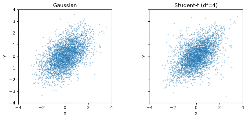
Holding the normal marginals and latent matrix fixed lets us see how changing the copula changes joint extremes. Identity Student-t shape would still not imply independence.

R = np.array([[1.0, 0.5], [0.5, 1.0]])
marginals = [ra.Normal("X", 0, 1), ra.Normal("Y", 0, 1)]
joints = {
    "Gaussian": ra.JointDistribution(marginals, ra.GaussianCopula(R)),
    "Student-t (df=4)": ra.JointDistribution(marginals, ra.StudentTCopula(R, df=4)),
}
fig, axes = plt.subplots(1, 2, figsize=(9, 4), sharex=True, sharey=True)
for ax, (name, joint) in zip(axes, joints.items()):
    sample = joint.rvs(3000, seed=2026)
    ax.scatter(*sample.T, s=3, alpha=0.3)
    ax.set(title=name, xlabel="X", ylabel="Y", xlim=(-4, 4), ylim=(-4, 4))
    ax.set_aspect("equal")
fig.tight_layout()
plt.show()
pd.DataFrame(
    {
        name: {
            "density at (1, 1)": joint.pdf([1, 1]),
            "CDF at (0, 0)": joint.cdf([0, 0]),
        }
        for name, joint in joints.items()
    }
).T

	density at (1, 1)	CDF at (0, 0)
Gaussian	0.094354	0.333333
Student-t (df=4)	0.106205	0.333328

Figure. Samples with identical normal marginals show different joint patterns for Gaussian, Student-t and Frank copulas; marginal distributions alone do not specify dependence.

Transform and recover physical points

For a Gaussian copula, canonical Rosenblatt and Cholesky Nataf are the same mapping. jacobian_u_wrt_x(u, x) returns \(\partial u/\partial x\), and jacobian_x_wrt_u(u, x) its inverse. Joint transformation methods take one vector; distribution methods accept rows of points. Copula-level Rosenblatt methods instead work on uniform coordinates.

joint = joints["Gaussian"]
nataf = joint.make_transformation("nataf")
rosenblatt = joint.make_transformation("rosenblatt")
x = np.array([1.2, -0.3])
u = nataf.x_to_u(x)
np.testing.assert_allclose(u, rosenblatt.x_to_u(x), atol=1e-12)
np.testing.assert_allclose(nataf.u_to_x(u), x, atol=1e-12)
J = nataf.jacobian_u_wrt_x(u, x)
np.testing.assert_allclose(joint.pdf(x), np.prod(norm.pdf(u)) * abs(np.linalg.det(J)))
print("Physical point:", x, "Normal point:", u)
print("du/dx:\n", J)

Physical point: [ 1.2 -0.3] Normal point: [ 1.2        -1.03923048]
du/dx:
 [[ 1.          0.        ]
 [-0.57735027  1.15470054]]

Reproduce the conditioning-order benchmark

Lebrun and Dutfoy (2009, Section 6) use exponential marginals with rates 1 and 3 and failure event

\[g(X_1,X_2)=8X_1+2X_2-1\leq 0.\]

For a Frank copula with \(\theta=10\), FORM gives approximately 0.107 in order \((X_1,X_2)\) and 0.122 in the reverse order. Exact probability is order-invariant; the first-order tangent approximation is not. The Gaussian copula with latent correlation 0.5 provides a comparison where orthogonal changes of normal coordinates preserve the optimum FORM result.

def exponential_model(copula):
    return ra.StochasticModel(
        ra.JointDistribution(
            [
                ra.ScipyDist("X1", expon(scale=1)),
                ra.ScipyDist("X2", expon(scale=1 / 3)),
            ],
            copula,
        )
    )


rows = []
for name, copula in [("Gaussian", ra.GaussianCopula(R)), ("Frank", ra.FrankCopula(10))]:
    choices = [("rosenblatt", [0, 1]), ("rosenblatt", [1, 0])]
    if name == "Gaussian":
        choices.insert(0, ("nataf", None))
    for method, order in choices:
        options = ra.FORMOptions(transform=method, rosenblatt_order=order)
        form = ra.FORM(
            model=exponential_model(copula),
            options=options,
            limit_state=ra.LimitState(lambda X1, X2: 8 * X1 + 2 * X2 - 1),
        )
        form_result = form.run()
        assert form_result.converged
        rows.append(
            {
                "Copula": name,
                "Method": method,
                "Order": str(order),
                "Beta": form_result.design_index,
                "FORM Pf": form_result.failure_probability,
            }
        )
results = pd.DataFrame(rows)
np.testing.assert_allclose(
    results.loc[results.Copula == "Frank", "FORM Pf"], [0.107, 0.122], atol=0.00015
)
results

	Copula	Method	Order	Beta	FORM Pf
0	Gaussian	nataf	None	1.295457	0.097581
1	Gaussian	rosenblatt	[0, 1]	1.295457	0.097581
2	Gaussian	rosenblatt	[1, 0]	1.295457	0.097581
3	Frank	rosenblatt	[0, 1]	1.242811	0.106969
4	Frank	rosenblatt	[1, 0]	1.165320	0.121945

We can integrate out \(X_2\) using the Frank conditional CDF. This gives an independent numerical reference for the event probability:

\[P_f=\int_0^{1/8}e^{-x}\,F_{X_2\mid X_1=x}((1-8x)/2)\,dx.\]

The plotted differences are FORM approximation errors, not changes to the specified distribution.

frank = ra.FrankCopula(10)


def integrand(x):
    p = [-np.expm1(-x), -np.expm1(-3 * (1 - 8 * x) / 2)]
    return np.exp(-x) * frank.rosenblatt(p)[1]


exact, quadrature_error = quad(integrand, 0, 1 / 8)
assert abs(exact - 0.1038) < 0.00005
print(
    f"Integrated Pf = {exact:.6f}; quadrature error estimate = {quadrature_error:.1e}"
)
fig, ax = plt.subplots(figsize=(6, 3))
frank_results = results[results.Copula == "Frank"]
ax.bar(["X1 then X2", "X2 then X1"], frank_results["FORM Pf"], width=0.5)
ax.axhline(exact, color="black", linestyle="--", label="Direct integration")
ax.set(ylabel="Failure probability", title="Frank copula: conditioning order and FORM")
ax.legend()
fig.tight_layout()
plt.show()

Integrated Pf = 0.103839; quadrature error estimate = 5.6e-10

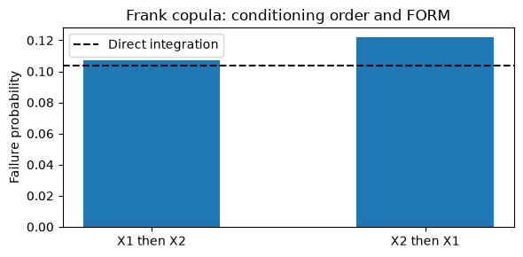
Figure. Frank-copula FORM probabilities change with conditioning order; the horizontal direct-integration reference represents the unchanged physical event.

Generalized Student-t Nataf: an exact half-space check

Choose Student-t marginals matching the copula’s degrees of freedom. The joint law is then multivariate Student-t. For \(g=3-X-Y\) and unit marginal scales,

\[\beta=\frac{3}{\sqrt{2+2\rho}},\qquad P_f=T_4(-\beta).\]

Generalized Nataf makes this event affine in spherical Student-t coordinates, so its FORM result is exact up to solver tolerance. These coordinates have identity shape, not independent components or unit covariance. get_equivalent_beta() converts the resulting probability to the conventional normal index.

student_joint = ra.JointDistribution(
    [ra.ScipyDist("X", t(4)), ra.ScipyDist("Y", t(4))], ra.StudentTCopula(R, df=4)
)
options = ra.FORMOptions(transform="nataf")
form = ra.FORM(
    model=ra.StochasticModel(student_joint),
    options=options,
    limit_state=ra.LimitState(lambda X, Y: 3 - X - Y),
)
form_result = form.run()
beta_exact = 3 / np.sqrt(2 + 2 * R[0, 1])
pf_exact = t.sf(beta_exact, 4)
np.testing.assert_allclose(form_result.failure_probability, pf_exact, rtol=2e-6)
pd.Series(
    {
        "Geometric beta (Student-t space)": form_result.design_index,
        "Normal-equivalent beta": form_result.beta,
        "FORM Pf": form_result.failure_probability,
        "Exact Pf": pf_exact,
    }
)

Geometric beta (Student-t space)    1.732051
Normal-equivalent beta              1.410804
FORM Pf                             0.079151
Exact Pf                            0.079151
dtype: float64

Choose the standard space for the analysis

An explicit Gaussian copula defaults to Nataf; Student-t and Frank default to normal Rosenblatt. System FORM, SORM, simulation methods and the strong maximum test currently require independent normal coordinates. Select Rosenblatt for these analyses with a non-Gaussian copula.

The following system has nested failure events, \(X>3\) and \(X>4\), so the series probability is exactly \(P(X>3)\). This checks the shared transformation used by the component analyses.

normal_margin_student = ra.StochasticModel(joints["Student-t (df=4)"])
system = ra.SeriesSystem(
    [
        ra.Component("threshold_3", lambda X: 3 - X),
        ra.Component("threshold_4", lambda X: 4 - X),
    ]
)
system_form = ra.SystemFORM(normal_margin_student, system)
system_form_result = system_form.run()
np.testing.assert_allclose(system_form_result.failure_probability, norm.sf(3), rtol=1e-5)
print("Standard space:", system_form_result.component_results["threshold_3"].standard_space)
print("System Pf:", system_form_result.failure_probability)

Standard space: normal
System Pf: 0.0013498980316286287

Continuous marginals and positive-definite elliptical shape matrices are required. Frank is currently bivariate with \(|\theta|\leq30\). Copula fitting and Pearson calibration for non-Gaussian copulas are not included. Finite precision limits extreme conditional probabilities; an unresolved transform raises rather than silently clipping coordinates.

For a practical component diagnostic, continue with the strong maximum test tutorial.

Continue with Rosenblatt ordering in system reliability for a worked reproduction of Meinen and Steenbergen (2025), including transformation geometry, consistent component coordinates, and direct probability checks.

Continue: User guide · API reference · Theory