Load Combination Distributions

Pystra includes a range of tools to enable the calculation of load combinations due to variable loads:

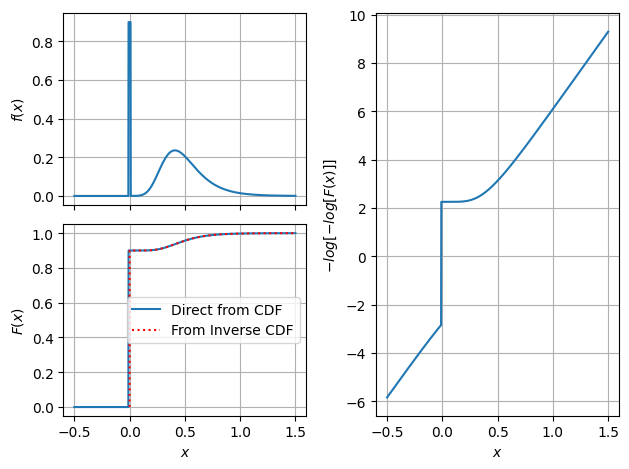
• Zero-Inflated Distributions allow for a probability of non-occurence of a load

• Maximum Distributions allow the distribution of maxima of a supplied parent or point-in-time distribution

• MaxParent Distribution allows the determination of the point-in-time distribution from a supplied maximum.

import pystra as ra
import numpy as np
from matplotlib import pyplot as plt

Zero-Inflated Distribution

zin = ra.ZeroInflated('Q',ra.Gumbel("G", 0.5, 0.2),p=0.9)
zin.zero_tol = 1e-2
x = np.linspace(-0.5,1.5,1000)
pdf = zin.pdf(x)
cdf = zin.cdf(x)
u = np.linspace(0,1,10001)
ppf = zin.ppf(u)
fig,axs = plt.subplot_mosaic([['a','c'],['b','c']],sharex=True)
ax = axs['a']
ax.plot(x,pdf)
ax.set_ylabel('$f(x)$')
ax.grid()
ax = axs['b']
ax.plot(x,cdf,label='Direct from CDF')
ax.plot(ppf,u,'r:',label='From Inverse CDF')
ax.set_ylabel('$F(x)$')
ax.set_xlabel('$x$')
ax.legend(loc='center right')
ax.grid()
ax = axs['c']
ax.plot(x,-np.log(-np.log(cdf)))
ax.set_ylabel('$-log[-log[F(x)]]$')
ax.set_xlabel('$x$')
ax.grid()
plt.tight_layout();
#fig.set_layout('tight');

def lsf(R,G,Q):
    return R - (G + Q)

def reliability(p=0.0):
    ls = ra.LimitState(lsf)
    sm = ra.StochasticModel()
    sm.addVariable(ra.Lognormal("R", 6.0,0.15))
    sm.addVariable(ra.Normal("G", 4.5, 0.2))

    g = ra.Gumbel("Q", 0.5, 0.2)
    if p == 1.0:
        sm.addVariable(ra.Constant("Q",0.0))
    elif p == 0.0:
        sm.addVariable(g)
    else:
        zig = ra.ZeroInflated("Q",g,p=p)
        sm.addVariable(zig)

    form = ra.Form(sm,ls)
    form.run()

    return form

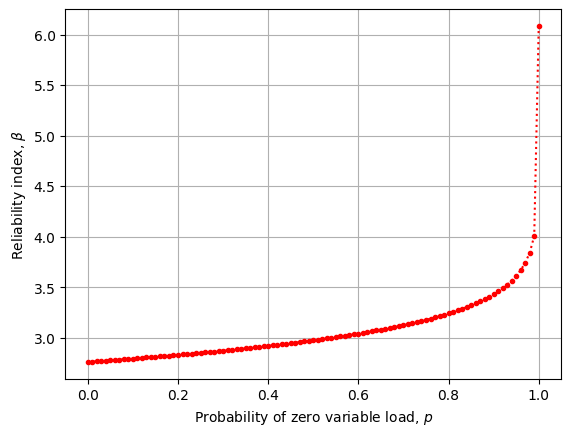
betas = []
ps = np.linspace(0,1.0,101)
for p in ps:
    form = reliability(p=p)
    betas.append(form.beta)

fig,ax = plt.subplots()
ax.plot(ps,betas,'r.:')
ax.set_xlabel('Probability of zero variable load, $p$')
ax.set_ylabel('Reliability index, $β$')
ax.grid();